Understanding AutoGrad From Scratch
Welcome to the very first tutorial of the series. This series of writeups is inspired by the fantastic video lecture series "Make More" by Andrej Karpathy. I am writing this series to get a much better understanding of all the foundational topics. In this first blog, we will understand the concept of AutoGrad. We will understand AutoGrad as a system or engine that computes automatic differentiation. We will not couple it with neural networks or deep learning-specific concepts. So, if you are unaware of Neural Nets, no worries. This blog is made keeping that in mind. In the next blog, we will brush up on all the essential theories of a neural network and build one from scratch using our AutoGrad engine. Finally, we will compare the results with PyTorch and see if it behaves the same as our AutoGrad engine. Sounds interesting. So, let’s get started.
The What and Why of AutoGrad
If you are familiar with neural networks, you know that training a neural network mainly comprises two phases. A forward step is when we calculate all the hidden states and the final predicted output of the network. In the backward step, we try to collect the gradient w.r.t the network’s loss to optimise the weights and hence the whole network. Computationally, it is very much impossible to calculate gradients of different functions comprising different operations by hand. So, we need a generalised algorithm that can automatically perform gradient calculation when given enough information about the network architecture (more about that below). AutoGrad is the solution to our above problem. This engine is designed to calculate and propagate the gradients throughout the network once we calculate the loss via the forward pass.
Understanding AutoGrad is essential; we often take PyTorch’s loss.backward for granted. However, there is so much going on under the hood. Usually, we rely on different abstractions while writing some logic. For example, array.sort() method is an abstraction for the sorting algorithm. However, it would make you highly nervous if you do not know how sorting works under the hood and use this abstraction and are given to implement something that needs high-performance sorting (with many edge cases). The same thing/phenomenon of leaky-abstraction could happen for backpropagation, too. So, re-inventing this wheel's micro (or nano) version could help us learn why and how things work.
Before you proceed
For this tutorial, you do not need to know how Neural networks work end to end; having basic knowledge or knowing something about neural networks surely helps. In this tutorial, we will not see in the eyes of Machine/Deep learning. We will perceive it as making an engine that automatically differentiates certain operations using the graph data structure.
So, for the sake of this tutorial, let’s define a neural network as an algorithm with two stages. The first stage is forward pass, where we do some arithmetic operations (see example 1, below). We stop the forward pass at some moment once we have defined our output variable. The second stage is called backward pass, where we devise a method that automatically derives the partial derivative of the output w.rt. all the variables we previously defined in our forward pass.
So all you need to know is the basics of derivatives and calculus and programming concepts like:
- How to compute derivative/partial derivative w.r.t. some variable
- Understand chain rule
- Object-oriented programming in Python
No worries. I will give you some pointers or resources for the portions of the topic that will use some of these tools.
The Computation Graph
Okay, let’s start with understanding what a computational graph means. Simply put, it means a graph-like data structure that keeps track of your sequential set of computations done over something. Let’s understand from an example:
a = 3
b = 4
c = a + b
d = c * c
e = d + a
f = e + 3
We have defined some sets of operations like addition and multiplication. The computational graph of all these operations w.r.t. the final variable f is shown below:
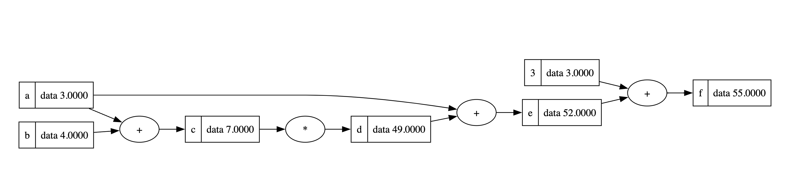
Figure 1: Computation Graph of a forward pass
The graph shows how each variable is dependent on each other operation-wise. Figure 1 shows the computation graph for the forward pass. However, as we learned before, in our backward pass, we would derive the gradient of the output f w.r.t. all the variables: a, b, c, d, e, f`. Let’s calculate the gradient manually first.
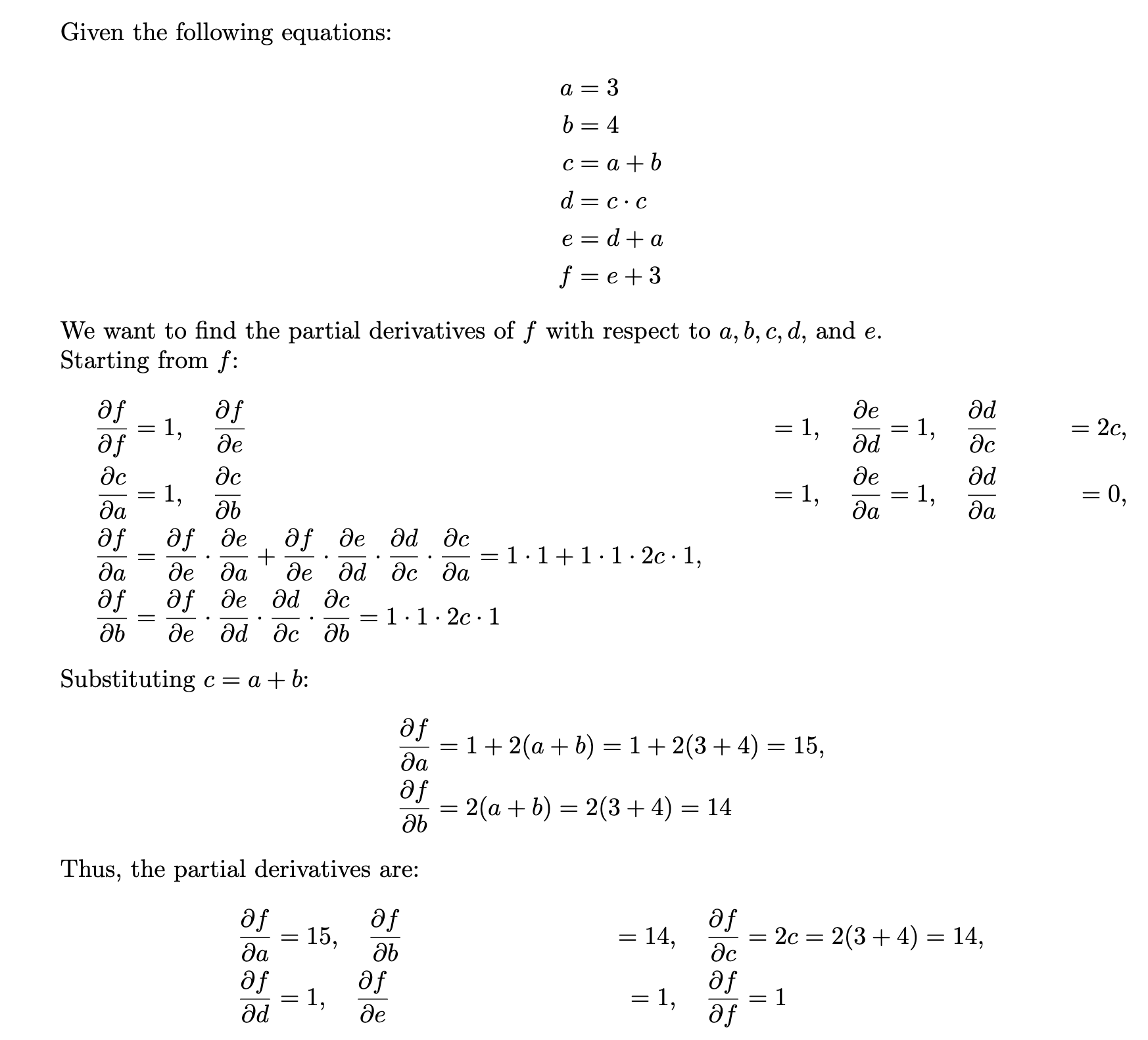
Figure 2: Manual Gradient Calculation by hand
Now let’s see how this look in our computation graph would look like for a backward pass.

Figure 3: Computation graph including backward pass (backward arrows drawn by hand)
The black lines shown here are the forward pass, and the red lines shown here are the backward pass. Next, we are going to build the same thing using Python. So, without further ado, let’s start.
Let’s build our computation graph
To build a computation graph, we need to think of the very atomic object, which can somehow store its value and keep track of its operation done to and its gradient (we will come to the gradient later). If we think of this in terms of the graph, then we can define a node as that atomic object that makes the whole graph and can store such information. Here, also we need to make something similar node a like object which will store the following things:
- It’s own value.
- The children node or the nodes that were used to create this node. For example, if we say
c = a + b, thencis the main node, and 'a' andbare the children nodes. However, a node does not always need to have children (for example:x = 3ory = 4). Those are the cases of a leaf node. - We also need to keep track of the operation done on the node. In the example above, we can say
+, or addition is the operation done on the nodesaandb. Whereas there were no operations done on the leaf nodesxandy. - Finally, keep track of the gradients w.r.t. the output. We will come back to this later. However, based on our above example, we need to keep track of values like
doutput/daordoutput/dxwhere output is some arbitrary value on which we will carry out our backpropagation.
So, the mindset would always be to define everything on a local basis, and the rest would be carried out recursively. What I meant by that is that you just need to define the properties of a single node, and then automatically, you will see that the computation graph has been created by itself.
The Value class
We will define a node, which will be a class that stores all the different properties. Let’s name the class Value. Please note that all the operations and manipulations that we are going to do here are done on zero-dimensional objects (or, in other words, just numbers). A very similar flow will be carried out on multi-dimensional objects or Tensor. However, that is out of the scope of this tutorial.
Now, let’s define our the bare skeleton of our Value class.
class Value:
    def __init__(self, data: int, label: str, _children = (), _op: str = ""):
        self.data = data
        self.label = label
        self._children = set(_children)
        self._op = _op

    def __repr__(self) -> str:
        return f"Value({self.label}, data={self.data})"
Super simple right? As mentioned earlier, this class holds its own value information stored in the variable data, _children will store the set of nodes (if any) that were used to create this very value object and _op will keep track of the operations between the current value object and its children. The method __repr__ is a special method that defines the string representation of the object. Let’s define a variable to see it in action.
a = Value(3, label="a")
print(a)

> Value(a, data=3)
We have defined a value object here. And since it does not have any _children or _op defined, so we can say, it is a leaf node.
If we have not defined the
__repr__method,print(a)would give a result like this:<**main**.Value object at 0x104946c00>.